The Ultimate Snapshot Report (part 3)

Hello there, yes, a third part of the snapshot report and I’m not even sure it’s the last one. The thing is that since the last post there has been some major improvements on the set up that I thought are worth sharing. In my previous post I ended up with a small defeat. There were some combinations of filters that when I drilled through to see all the historic records of those order IDs I would not get any rows. Also my set up included duplicating the fact table which is a big no-no in most use cases and a shameful solution from a modeler perspective. Even though this was the best I had, I decided to present the topic on two events, one was the Data Community Day Austria 2023 and the other was @PowerBIEspanol Virtual Conf 2023 (Fin Tour Power BI Days), just a few days apart. The fact that I had to present the solution to a lot of people kept me thinking and looking for solutions, so with the help of the always reliable Ricardo Rincón I finally found out a working solution just duplicating dimension tables and creating dimension tables for everything (even comments and stuff like that). That was much better but not quite scalable. In real life things are ugly and tables have many columns. So while fighting with the same use case at work, I found a sneakier and much better solution that got rid of all those superfluous dimension tables reducing the need of them to just 2. While preparing the presentations I also worked a bit on the report layer and I’ll also share some techniques I came up with that can be helpful at some point. But enough of all this talking, let’s do what? Let’s get to it.
The Report
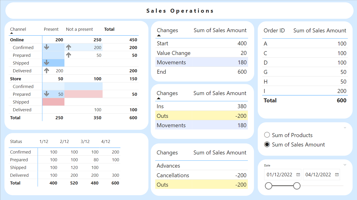
As you can see I did some improvements on the reporting layer. Far from perfect, at least now looks half decent. The use case and the logic behind the numbers is the same as in the previous blog post so I will not go into the details again. When no filter is selected, the top left matrix shows the status on the last snapshot of the selected range, but this time I added some conditional formatting to add more information. We’ll get into that later. The table underneath shows aggregated values per date in the selected range. The three tables in the middle explain how we got from the first snapshopt to the last one selected, analying it at three diferent levels. The middle table shows a break down of ‘Movements’, and the bottom table shows a break down of ‘Outs’. Finally the top right table shows a detail of order Ids and below that there is a field parameter to switch between units and sales amout and finally the date filter to select the range of snapshots to analyze.
Interacting with the report
Interacting with this report is fun because you can really get to the bottom of any value you see. If you click on the dates of the bottom left table you can see the snapshot of that day, if you click on the Changes items you can see in which filter combinations happened and even on which dates. And if you want to know the whole story of any group of order Ids you can always drill through and see the whole history of those ids. Quite proud of it after all the DAX tears I have shed for this use case.
Switching between a date range and the latest snapshot of the range
This is already an improvement over the previous blog post. Here I used to filter with a calculated column that would retrieve always the latest snapshot of the fact table, but later I realized that this did not work well if a user wanted to analyze a range of snapshots that did not include that last snapshot. So here I kept the two calendar tables, but I added a calculation group that would capture the last date of the date range (defined in ‘Date 2’) and apply it if it came from the regular ‘Date’ table. Since I came up with this idea later on the design process this is implemented as «Model 2» calculation group:
-------------------------------
-- Calculation Group: 'Model 2'
-------------------------------
CALCULATIONGROUP 'Model 2'[Model 2]
    Precedence = 40

    CALCULATIONITEM "Last Date in Range" =
        VAR maxDate =
            MAX ( 'Date 2'[Date] )
        VAR result =
            CALCULATE ( SELECTEDMEASURE (), TREATAS ( { maxDate }, 'Date'[Date] ) )
        RETURN
            result
An important bit here is that the precedence of this calc group must be higher than the «Changes» calc group we saw in detail in the previous blog post. This way it is easy to remove the filtering from the «Date» table and recover again the whole date range. The top left matrix and the top right table have this calculation item applied at the visual level, so by default they show data from the latest snapshot, but this filtering is removed when a calc item from the «changes» calc group cross filters them. In the previous implementation I had yet another calc group in charge of removing filters on the date table anad this was applied at the visual level filter in all the central tables to achieve the effect I just described. However after several DAX fights I decided to take care of that within the calc items themselves to simplify the overall structure and ease my calc group precedence nightmares.
Conditional formating on blank cells
This is something I did not expect and took some effort to find a workaround. Conditional formatting is only applied in non-blank cells. Even if the measures you are using for conditional formatting are not blank, no formatting will be applied if the measure that is showing the actual value of the cell is blank for those filters. That was a problem in my case because I wanted to show conditional formatting in all cells, regardless of the value. There may be no orders now in Shipped status, but I want to tell the user if the number of orders in that status has grown or decreased over the period. Of course the first thought was to use a calc group at the visual level to add a 0 to the SELECTEDMEASURE so that I would always have a value. The Zeros are ugly, but you can get rid of them with some format string wizardy:
0;-0;;
A format string like this will hide the zeros. Howeveer there was another problem. If you add a calculation group to achieve this, this transformation becomes part of the filter context, and as such it will travel when you crossfilter or you do a drill through. And that’s terrible, because then you will always see all orders, not just the relevant ones. So I had to think harder. The workaround I found was to create two new measures that were equal to the two measures I had (Number of Products and Sales Amount) but adding a +0 at the end.
------------------------------------
-- Measure: [Sum of Products plus 0]
------------------------------------
MEASURE 'Orders'[Sum of Products plus 0] = [Sum of Products] + 0
    FormatString = "0;-0;;"

----------------------------------------
-- Measure: [Sum of Sales Amount plus 0]
----------------------------------------
MEASURE 'Orders'[Sum of Sales Amount plus 0] = [Sum of Sales Amount] + 0
    FormatString = "0;-0;;"
Next, I created a field parameter including this two new measures in the same order as on my existing field parameter, and then I created a relationship by the order column!
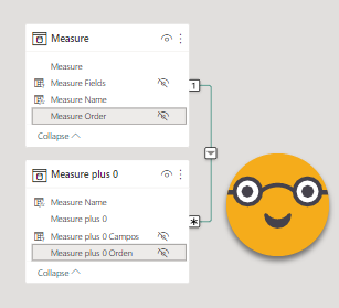
And then I modified the field parameter that was being used in the top left matrix, and left the orignal one in the rest of visuals.
Conditional formatting using calculation groups
The conditional formatting itself deserves a section because it had me puzzled for a while. My objective was to show with arrows if the value on a cell had increased or decreased between the initial and final snapshot. Then with colors I wanted to show if there are more cencellations than advancements (in red) or more advancements than cancellations (in blue) or it was balanced (white). Since I wanted to use the same logic I had on the calculation items I thought, well, why not reuse them? After all I had some filtering in my calc items so that only the two measures of the field parameter would be affected. Oh and now that we talk about this, of course I had to modify my calc items to acto on the «measures plus zero» as well. All calc tiems follow this structure
CALCULATIONGROUP 'Changes'[Changes]

    CALCULATIONITEM "Start" =
        IF (
            SELECTEDMEASURENAME ()
                IN UNION (
                    VALUES ( 'Measure'[Measure Name] ),
                    VALUES ( 'Measure plus 0'[Measure Name] )
                ),
            <code>,
            SELECTEDMEASURE ()
        )
This gave me a sense of security that the calculation item would not affect my conditional format measures. I WAS SO WRONG. My conditional format measure looked like this:
-----------------------------------------
-- Measure: [Sales Amount Ins vs Outs CF]
-----------------------------------------
MEASURE 'Changes'[Sales Amount Ins vs Outs CF] =
    VAR Movements =
        CALCULATE ( [Sum of Sales Amount], 'Changes'[Changes] = "Movements" )
    VAR result =
        SWITCH ( TRUE (), Movements > 0, 1, Movements < 0, -1, 0 )
    RETURN
        result
But then sometiems when I crossfiltered from the Changes table in the middle I would see changes in the conditional formatting which made no sense. If my measure is not one of the measures in the field paramters, why is it being affected?!? Well, because breaks one the sacred laws of calc groups: «Thou shalt not apply twice the same calculation item.» When you get to the IF statement you are already applying the calculation item, even if the result is «SELECTEDMEASURE()». It’s obvious, but I fell for that. It was a humbling experience to break the sacred rule after so many sessions on calc groups to be honest, but once I realized what was going the solution was just a few clicks away. I just went into Tabular Editor and duplicated the calc item and added a «CF» at the end of the calc item name to make it explicit that it’s just for conditional formatting. Just modifying the calc item used in the conditional format measure solved the issue. Hoooray! When setting the conditional formatting you need to do it for each of the measures of the field parameter.
The «Changes» calc group
Most of the calc group has stayed mostly the same, I just modified the initial filtering by measure name as explained above and then I included the REMOVE filters on the ‘Date’ table instead of relying on a calc group to do it. Please download the pbix file from the end of the article to look at the details.
Getting to see all records for relevant order IDs
As I mentioned in the previous post, this is a very thorny problem, even though in my head it looked easy at first. Pick up the relevant order ids, and then remove all filters and apply the filter on the order id column. Then you get all the records from them. The thing is that if you use any columns from the fact table on the detail table, there’s no way you will be able to expand the filter context with just DAX, because the filter context created by these columns is affected by the original filters. After all, the evaluation happens inside the filter context created by the columns of the fact table you are using in the detail table. So when you pick up the relevant order Ids, for those rows you will get no order id, because that record was not included in the orignal filter context, that’s why. Took me a lot of pain and debugging to finally see that.
So, you can’t use columns from the fact table in the detail table if you want to do this sort of drill through. So what are you going to do? One way is «All fact table columns move to dimensions no-matter-what». But this is a huge overhead for the model for just that. Still better than replicating the fact table like in my previous post, but still.
When I found myself having to do that with the big ugly model in my current client, I thought a bit more if I could do something else. And I found something that works! In this approach you still need the Order ID Dimension and yet another Date table, but that’s it, with these two columns you can identify each row of the fact table. For all the different attributes of the fact table, instead of using the columns of the fact table, you can use MEASURES! Yes, once you have the date and the order Id, you can just do a LOOKUPVALUE and go grab the value of that column for that order ID and DATE without worrying about the filter context!
So to recap, for the detail table you need:
- A new date table
- An order ID dimension
- A calculation group to extract the relevant order IDs and remove the effect of the original filter context
- A bunch of measures to show values fromthe fact table columns
- Copies of the measures to avoid interference from the Changes calc group
The calculation group looks like this:
-----------------------------
-- Calculation Group: 'Model'
-----------------------------
CALCULATIONGROUP 'Model'[Model]
    Precedence = 30

    CALCULATIONITEM "Order ID Hist v2" =
        VAR orderIDs =
            CALCULATETABLE (
                SELECTCOLUMNS (
                    FILTER (
                        ADDCOLUMNS ( VALUES ( 'Order ID'[Order ID] ), "@v", [Sum of Sales Amount] ),
                        [@v] <> BLANK ()
                    ),
                    "Ids", 'Order ID'[Order ID]
                ),
                REMOVEFILTERS ( 'Date 3' )
            )
        VAR fullHist =
            CALCULATE (
                SELECTEDMEASURE (),
                orderIDs,
                REMOVEFILTERS ( 'Present' ),
                REMOVEFILTERS ( 'Status' ),
                REMOVEFILTERS ( 'Channel' ),
                REMOVEFILTERS ( 'Date' ),
                REMOVEFILTERS ( 'Date 2' )
            )
        RETURN
            fullHist
When defining orderIDs variable we capture all relevant order ids and then we evaluate the measure (which we’ll make sure is not affected by the Changes calc group) and removing the effect of the original filter context. And yes, the original fitler context must be set up exclusively by dimensions so that you can efectively remove their effect on the fact table. Important bit is also the REMOVEFILTERS on the ‘Date 3’ table so that it does not interfere with the filter context of the first
Now what about those lookup measures? They look like this
---------------------
-- Measure: [Channel]
---------------------
MEASURE 'Lookup Measures'[Channel] =
    VAR currentDate =
        SELECTEDVALUE ( 'Date 3'[Date] )
    VAR currentOrderID =
        SELECTEDVALUE ( 'Order ID'[Order ID] )
    VAR result =
        LOOKUPVALUE (
            'Orders'[Channel],
            'Orders'[Date], currentDate,
            'Orders'[Order ID], currentOrderID
        )
    RETURN
        result
I created a measure table to put them in. You might want to hide them in production not to confuse people around. Basically we take the values from the two dimension tables that we use on the detail table and with tme we have the all we need to go grab the value of the rest of the columns. Each measure goes pick up a different column.
To show the Sum of Products and and Sales Amount, you do need a copy of the measure so that the calc item will not affect their value. We just need a measure with a different name, so you can just go:
-----------------------------------
-- Measure: [Sum of Sales Amount 2]
-----------------------------------
MEASURE 'Orders'[Sum of Sales Amount 2] = [Sum of Sales Amount]
    FormatString = "0"
Now if you build your detail table this way (and you build the visuals on the main report page using only dimension columns for filtering!) you’ll be able to drill trhough and see all the records for those IDs, and that may even go further than the range of dates selected.
While you are at it you can also add a remove filters button if you suddently want to see all records of all order ids to filter them in another way
And with that I think I summarize everything that I wanted to share about this model and report. Download it and play around with it. It’s not the fastest model on earth, but it gives the value, which is the first requirement, remember. Value change, Advancements and Cancellations are the 3 most «expensive» calc items in terms of of performance, but the logic is quite tricky. Like everything else it can be optimised, but with the correct value I’m happy enough at this time.
Download the pbix here
And follow the conversation on Twitter and LinkedIn
Thank you for reading!