Hi there. In my previous post on how to set up a «data problems» button I did mention that there was a further improvement to the approach, so here I am to explain what is this about.

As you may recall, in my previous installment on the topic, the user is warned that there is some issue with the data through a button that brings him or her to a page where can see exactly what are the issues, such as unmapped items or any other data issues (dates which are not dates, numbers which are not numbers, duplicates…). Today will stick with the mapping problems. In such case you had to copy the offending items, add them to the excel table, and complete the (manually maintained) extended attribute columns.

Wouldn’t it be wonderful if those items could automatically travel to the excel file?

Well, this is exactly what we’ll try to get to in this post. We are going to do data mapping with table connected to the dataset

This technique is not my idea, is from Denis Corsini, but I got his permission to blog about it. He may publicly post it in the future, in which case I’ll link it so you can go to the source of things. He calls it «The Circular Model»

The basic idea is that we’ll create a query to the dataset from Excel, where we’ll inform the extra column we’ll have added. Then we’ll add the excel as an extra source and modify the query use the column from the excel file.

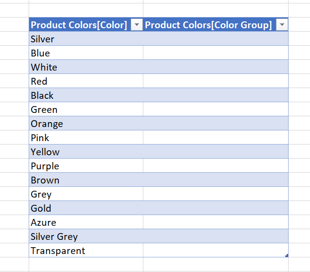
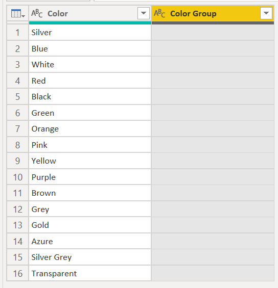
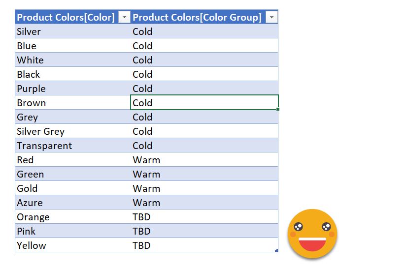
Let’s go step by step. First of all we’ll create a column, either with DAX or Power Query as if it all was nice and done. Following the example of the previous installment, we’ll imagine we have a table with all colors, and a color group column, by default blank. The crucial part is that the color column comes from the source data, so that if new colors appear they will be in this table too.

Starting from the Product Table, we’ll remove all but the color column, remove duplicates, and add the extra column. Very straight forward.

let
  Source                   = Product,
  #"Removed Other Columns" = Table.SelectColumns(Source, {"Color"}),
  #"Removed Duplicates"    = Table.Distinct(#"Removed Other Columns"),
  #"Added Custom"          = Table.AddColumn(#"Removed Duplicates", "Color Group", each "")
in
  #"Added Custom"

Going this way, we’ll need to keep the table to the model because this will be the table that we’ll be querying from Excel. If you do not want to keep this table, it is possible, we’ll just need to change a little bit the DAX query that will read from the dataset. We’ll see this latter option later on this post.

Now it’s time to publish to the service. Once published we’ll click on Analyze in Excel option either from the workspace view or from the report view.

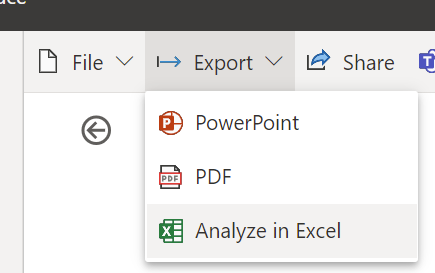
If it’s the first time, download the drivers or whatever it tells you to install. If you already did this, click on the small link underneath.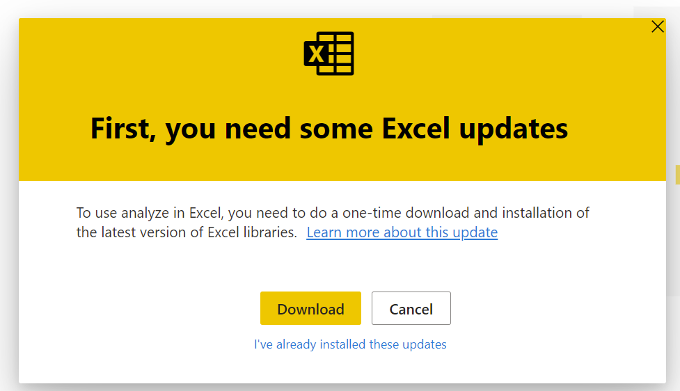

We’re getting now on the techiest part of it. We open the excel file (enable editing, enable data connections), go to connections & queries, select the only connection there is and click export. It will save the connection file in your hard drive. Save it wherever you like and open it with a text editor such as notepad or notepad++.

Look for the items marked in blue

…
<meta name=ProgId content=ODC.Cube>
…
<odc:CommandType>Cube</odc:CommandType>
<odc:CommandText>Model</odc:CommandText>
…

And change them to

...
<meta name=ProgId content=ODC.Table>
... 
<odc:CommandType>Default</odc:CommandType>
<odc:CommandText>EVALUATE 'Product Colors'</odc:CommandText>
...

Here EVALUATE ‘Product Colors’ is the dax query that we’ll be using. It just needs to be a valid dax query since we’ll be able to change it later if we wish to do so.

Save the file and close it.

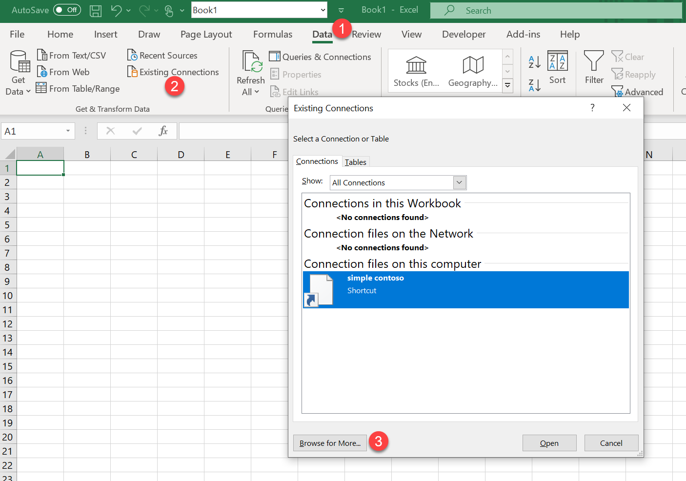
Now open a new excel file, go to data (1), existing connections (2), browse for more (3)

Now select your file and make sure you add it as a new table

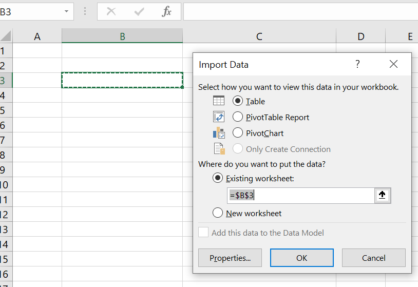
click ok and bam, here’s our table. About the headers I don’t know any way of getting rid of the square brackets. If you specify column names at least you don’t get the table name, but that’s about it, the square brackets remain. (let me know if you have a way)

This table really is connected. You can test by modifying it and then refreshing (right click on it + refresh, or many other ways of doing it). Anything you did to it will just disappear.

But what’s the point then?

What we’ll do now is add this table into the model. And I don’t mean the ‘Product Colors’ table into the model. We are querying it after all. What I mean is the table from the excel file, which will have manual inputs! and then will tweak the Product Colors table to include all what we already entered. But not so fast. Now we’ll put the excel file on a sharepoint. But before we do that there’s something that bugs me and that’s the fact that the connection is stored in a file in my hard drive, so I’ll just modify the query a liiitle bit. Actually just breaking it into two lines is enough to get the following message.

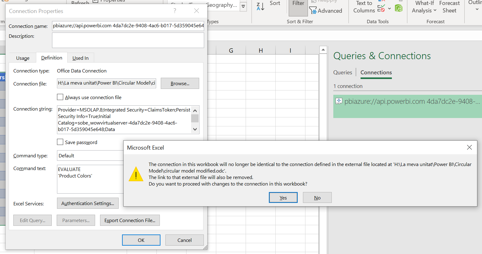
Well since breaking the link it’s what we wanted let’s say yes, save the file and move it to sharepoint, from where we’ll be able to update. Before doing that though, we might as well give a proper table name, sheet name and hide the gridlines, right?

Ok, the file is in a sharepoint, so we just need to go to Power BI desktop and add a new source from sharepoint folder. But before that…

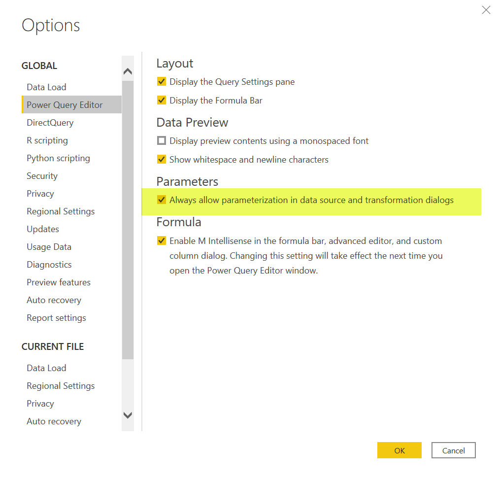
This post might get too long, but I want to share how I do it in case you find it useful. First of all, you need to enable the setting to allow to use parameters always:

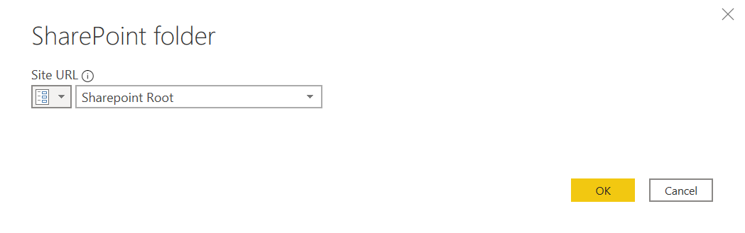
This will get handy in a minute. When we finally go to add new source –> sharepoint folder, now we can specify the URL from a parameter. Since we do not have any parameter with the URL we want to use we just go to «New Parameter» …

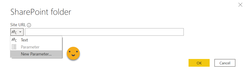
… and we give it a name, specify text type and type in the URL of our SharePoint site.

 

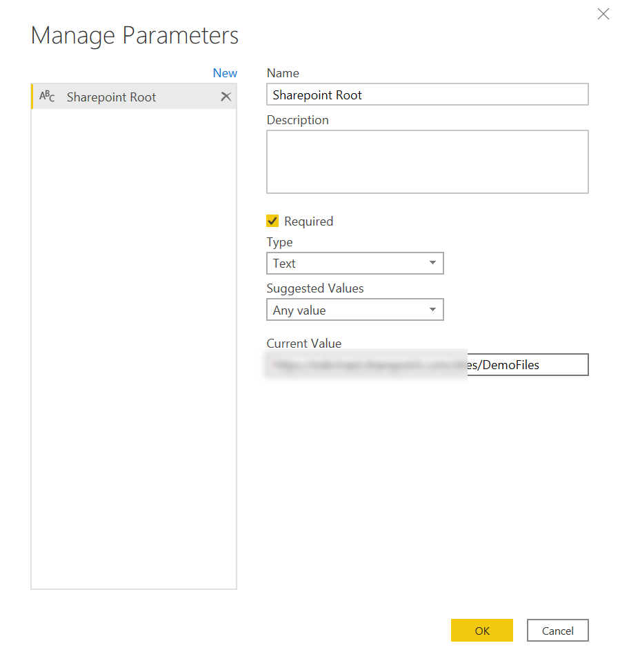
When we click OK we return to the previous dialog with the parameter already selected for us.

This might seem like extra work for little gain, but wait a minute!

On the next screen we are asked if we want to load the file list as a table (which is of no use 100% of the time since some columns cannot be loaded as they are and who needs a file list for their reporting anyway), so we click transform data and we get again the file list but now we can do something about it.

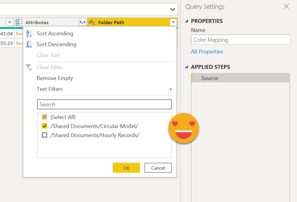
Sharepoint files can get very crowded, so first thing is to filter by the folder where your file is (to avoid picking up files with the same name somewhere else like a backup folder or whatever). The problem, for me, is that the folder path is ridiculously long, and it creates a dependency on the absolute path of the site. So I just remove the root path to keep the relative path. And now the parameter comes handy.

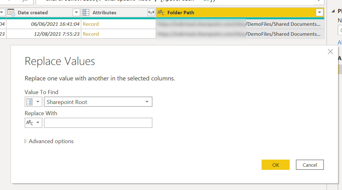
So we have this beautiful view with just the relative path to each of the files in the sharepoint site. If we ever have to move the sharepoint  site to another address we just need to change the parameter value. Also, since this query at this point might come in handy later if we need to get another file form the same sharepoint file, we’ll call it «SharePoint Root Folder» or something like that and we’ll disable loading.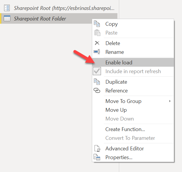

Now to continue with our query will click on «Reference» from the same contextual menu and we’ll get a query that starts where this one ends. We’ll give it a name and filter by the folder where our file is. By the way, put files in folders, not all together. Sooo easy to select the folder now.

If you do a lot of work with sharepoint sources, this comes handy! really. While you are at it, since we are getting to one file, add it as a step even if you have only one file, it will make your query robust towards other files that people might through in the folder, such as manuals and the like.

so finally we have our file and we can just expand it and go to the table with our data.

the M code to reach it is something like: (I’m no power query jedi, don’t judge me)

let
  Source = #"Sharepoint Root Folder", 
  #"Filtered Rows" = Table.SelectRows(
    Source, 
    each ([Folder Path] = "/Shared Documents/Circular Model/")
  ), 
  #"Filtered Rows2" = Table.SelectRows(
    #"Filtered Rows", 
    each [Name] = "Circular Model color Input.xlsx"
  ), 
  Content = #"Filtered Rows2"{0}[Content], 
  #"Imported Excel Workbook" = Excel.Workbook(Content), 
  #"Filtered Rows1" = Table.SelectRows(#"Imported Excel Workbook", each ([Kind] = "Table")), 
  ColorMapping_Table = #"Filtered Rows1"{[Item = "ColorMapping", Kind = "Table"]}[Data]
in
  ColorMapping_Table

If you want you can change the headers, but really it does not matter too much since we’ll not be loading this table, just merging it with the one we are now querying from the excel. Before we forget, let’s disable loading from this new query.

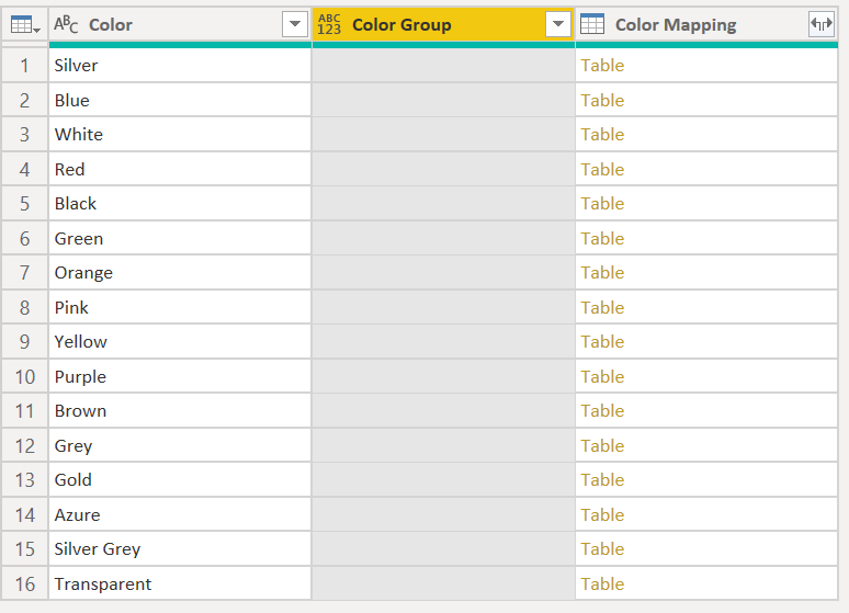
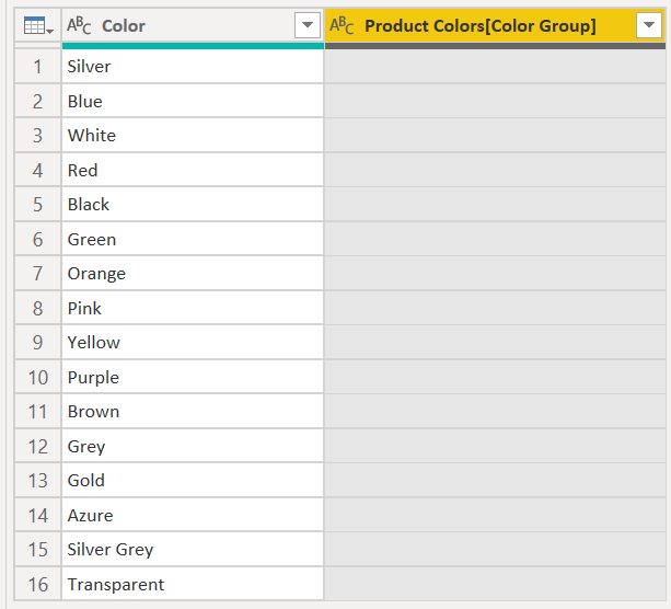
Now we can merge it with the original Product Colors

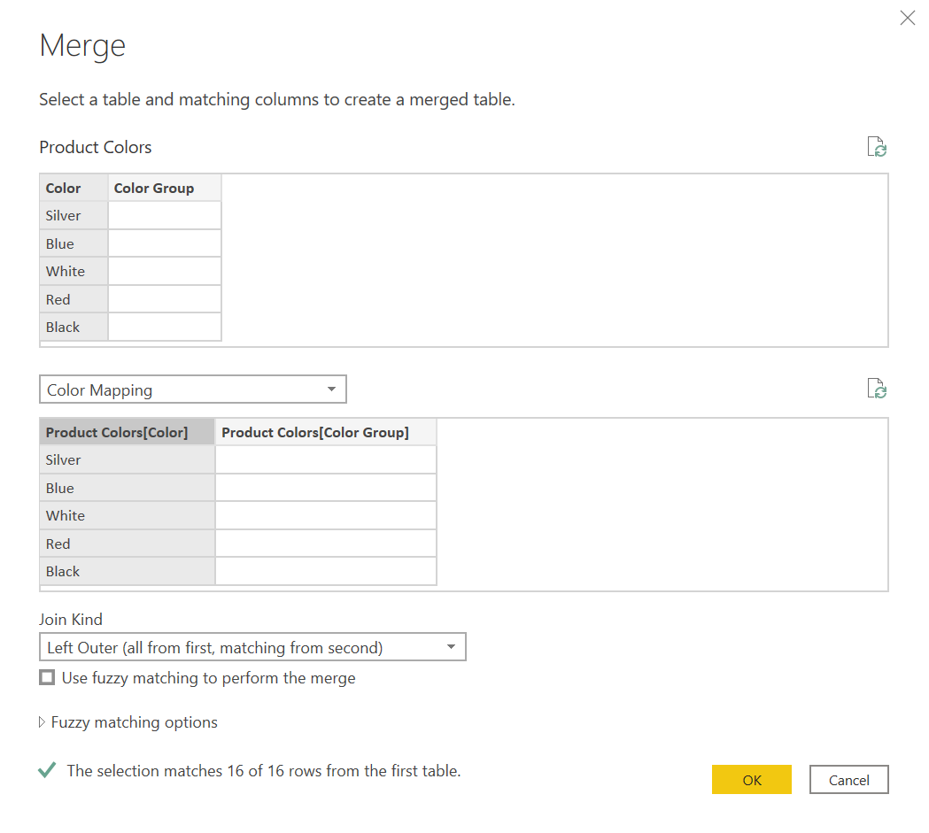
And we’ll just replace the existing «Color Group» column, with the column coming from the ColorMapping table, which we’ll rename to «Color group» at the end:

Expand:

Add only the new column

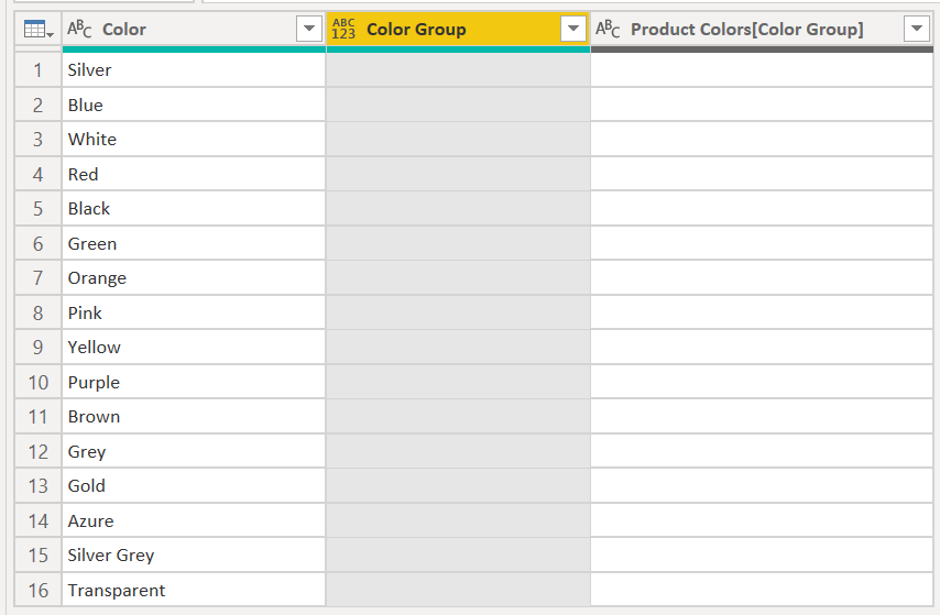
Remove the original column

Rename the new column to match the original one

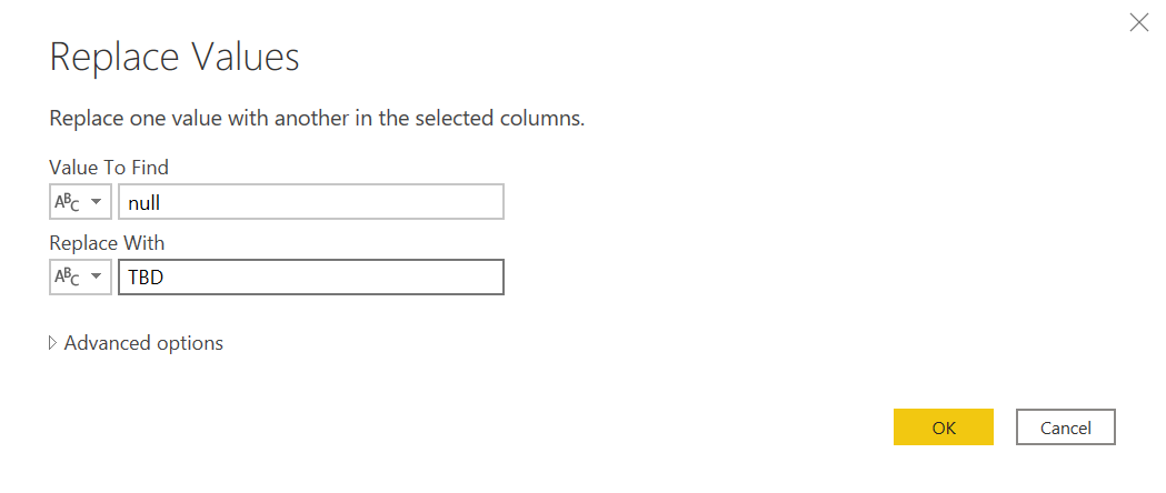
Now we might want to give blank mappings some actual text, such as «TBD» (To be defined). We can replace blanks with such text. We aware that a blank cell from excel will show as empty string, while a color not present in the excel table will result in null.

So we’ll need 2 steps (or some more advanced M skills)

 

And that’s it!

How can we test it?

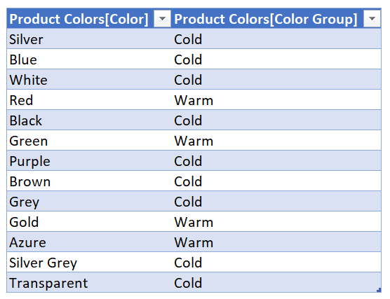
To make it a bit more realistic we’ll delete a 3 rows from the excel table (on the sharepoint folder) and map all the rest with either warm or cold color.

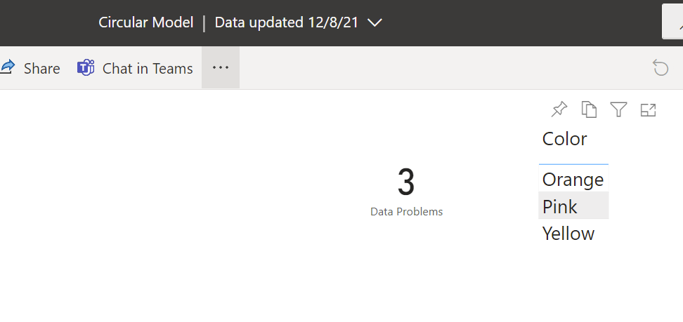
Now we’ll publish the dataset and refresh it so that the mapping will be included in the dataset from which the excel file reads. Depending on your setup you’ll need to put your credentials on the different data sources as usual before you can refresh from the service. But once it works, you’ll see that the report shows there are 3 data problems! Orange, Pink and Yellow are not mapped (for details on how to set up such a «data problems» sheet check out the post I mentioned at the beginning)

So now we would go to the excel on the sharepoint (we can even put a link on this report page to remove all friction) and we need to refresh the table. At least on my end it didn’t work from Excel Online (even though pivot tables do refresh!) so we’ll need to open the Excel file from sharepoint on the desktop app to be able to refresh.

But when we do… indeed! here they are! no copy paste involved.

Since we are editing a file from sharepoint we just need to update the TBD’s for either «Warm» or «Cold», save and we are good to go! on the next refresh these extra colors will be mapped. And since they com straight from the source there are no typo problems. There might be capitalization issues though as we discovered in the previous post on data mapping cited already twice (not pasting the link for the third time)

And that’s pretty much it!

If you want to skip the extra Product Colors table, you just need to create the Color Group column in the Product table and to modify the dax query to

SUMMARIZE( 'Product', 'Product'[Color], 'Product'[Color Group] )

And then later replace it with the column coming from the excel file in a similar fashion of what we did.

Is it quick? Maybe not. Is it better than just mapping bare-back copying and pasting values as they show up?  Definitely. Which way we should go? As usual, it depends. For serious projects, I recommend this approach.

The only thing worth noting is that you should definitely not enable refresh on open for the excel file. Because if you refresh the excel before the last changes have been loaded to the dataset your beautiful edits will revert to the last copy that was loaded to the dataset.

Also, this works well for ever-larger datasets. If you want to map items from a snapshot that will contain more or less items in each load, this might not be the right approach. But then again in BI normally we’ll keep history so this should not be a big problem. Even in such case you might still get away reading from both the source table and the table coming from the excel file (you’ll need to keep it in your dataset) but the dax query will be trickier.

If you read up until here, kudos to you. I appreciate it.

 

[bws_google_captcha]